Classifying my Own Images

When I was an undergraduate, I kept a diary of my daily life and I’ve always wanted to digitise it, to keep it safe. I kept it over the course of five years, and I have scanned in a limited number of pages (so far). As mentioned, as a long-term goal, I’d quite like to digitise the written words into plain text. But for now, the scanned images provide a useful resource with which to practise my machine learning skills. You can see an example scan above.

I wrote a quick Python program to split these images into left and right pages (with the split point selected manually), to give 700 x 1000 pixel images.

My aim was to build a Keras model using ConvNets which would be able to determine whether a given page is a left or right page: a simple binary classification problem.

Reading the Images into Python

The first step in this process was to read the images from files on my computer into tensors, suitable for processing by the Keras model. I also needed to create a training set, a validation set and a test set with labels (left or right), to be used for training and then assessing the model.

I have recently read about Python Generators in the excellent “Deep Learning with Python” book (François Chollet, published by Manning), in particular the ImageDataGenerator provided as part of Keras. This provides a means of reading the images into input tensors with many different options, I used the mechanism that also infers the labels from the directory structure that you provide.

I created the following directory structure for use by the generator and placed the images in the correct locations. I split my 320 images into three sets (allocated randomly): training (240), validation (40) and test (40). Each of these was then divided into left and right directories.

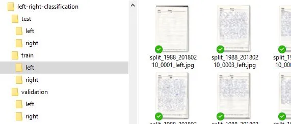
A generator is then created as in the following code block, it will be used later to train the model using the fit_generator (instead of “fit”) function of the model. In a similar manner the validation and test generators were also created.

batch_size = 10
train_datagen = ImageDataGenerator(rescale=1./255)
train_generator = train_datagen.flow_from_directory(
                                                directory="images\\" + image_path + "\\train",
                                                class_mode="binary",
                                                target_size=(500, 350),
                                                classes=["left","right"],
                                                batch_size=batch_size,
                                                shuffle=True)

This code first converts the [0 to 255] RGB values of the images to [0.0 to 1.0] and also reduces their size to 350 x 500 in order to reduce the model size. Other transformations can also be applied by ImageDataGenerator, allowing it to be used for data augmentation (that is, creating extra training data by transforming the same images in some way and adding them to the data).

Remember, image dimensions are usually represented as width x height (e.g. 350 x 500) whereas Python NumPy arrays are described as (rows, columns) (e.g. target_size=(500, 350)). A bit confusing, but I think we can cope!

The Model

As these are images, I decided to use ConvNets to process them (although this is such a simple problem that straight Dense layers may have sufficed). For a first attempt, I added two ConvNet layers, with Max Pooling in-between, followed by a Dense layer before the final single-node classifier. Here’s the code.

model = models.Sequential()
model.add(layers.Conv2D(32, (3,3), activation="relu", input_shape=(500, 350, 3)))
model.add(layers.MaxPooling2D((2,2)))
model.add(layers.Conv2D(64, (3,3), activation="relu"))
model.add(layers.MaxPooling2D((2,2)))
model.add(layers.Flatten())
model.add(layers.Dense(256, activation="relu"))
model.add(layers.Dense(1, activation="sigmoid"))

Compiling and Training the Model

As mentioned earlier, I used the fit_generator function to train the model. My first attempts at running this code resulted in an accuracy of 0.5, which meant that the model was no better than chance. After checking my code, I started tweaking the learning rate and eventually found the best value for the validation set.

num_train_images = 240
num_val_images = 40
steps_per_epoch = num_train_images / batch_size
val_steps_per_epoch = num_val_images / batch_size
learning_rate = 0.00001                                     # tune this!

model.summary()

model.compile(loss="binary_crossentropy", optimizer=optimizers.rmsprop(lr=learning_rate), metrics=["acc"])

history = model.fit_generator(train_generator, steps_per_epoch=steps_per_epoch, epochs=30, validation_data=validation_generator, validation_steps=val_steps_per_epoch, shuffle=True)

# Save the trained model for later use
model.save("left_right_page_v2.h5")

Here’s the output.

Using TensorFlow backend.
Found 40 images belonging to 2 classes.
Found 240 images belonging to 2 classes.
_________________________________________________________________
Layer (type)                 Output Shape              Param #
=================================================================
conv2d_1 (Conv2D)            (None, 498, 348, 32)      896
_________________________________________________________________
max_pooling2d_1 (MaxPooling2 (None, 249, 174, 32)      0
_________________________________________________________________
conv2d_2 (Conv2D)            (None, 247, 172, 64)      18496
_________________________________________________________________
max_pooling2d_2 (MaxPooling2 (None, 123, 86, 64)       0
_________________________________________________________________
flatten_1 (Flatten)          (None, 676992)            0
_________________________________________________________________
dense_1 (Dense)              (None, 256)               173310208
_________________________________________________________________
dense_2 (Dense)              (None, 1)                 257
=================================================================
Total params: 173,329,857
Trainable params: 173,329,857
Non-trainable params: 0
_________________________________________________________________
Epoch 1/30
2019-02-17 13:46:29.456091: I tensorflow/core/platform/cpu_feature_guard.cc:141] Your CPU supports instructions that this TensorFlow binary was not compiled to use: AVX2
24/24 [==============================] - 72s 3s/step - loss: 0.8597 - acc: 0.5375 - val_loss: 0.6948 - val_acc: 0.5000
Epoch 2/30
24/24 [==============================] - 66s 3s/step - loss: 0.6978 - acc: 0.5417 - val_loss: 0.7016 - val_acc: 0.5000
Epoch 3/30
24/24 [==============================] - 66s 3s/step - loss: 0.6820 - acc: 0.5792 - val_loss: 0.6656 - val_acc: 0.7750
Epoch 4/30
24/24 [==============================] - 66s 3s/step - loss: 0.6754 - acc: 0.5625 - val_loss: 0.6561 - val_acc: 0.5000
Epoch 5/30
24/24 [==============================] - 66s 3s/step - loss: 0.6678 - acc: 0.5583 - val_loss: 0.6603 - val_acc: 0.5000
Epoch 6/30
24/24 [==============================] - 66s 3s/step - loss: 0.6502 - acc: 0.6167 - val_loss: 0.6397 - val_acc: 0.5000
Epoch 7/30
24/24 [==============================] - 65s 3s/step - loss: 0.6351 - acc: 0.6875 - val_loss: 0.6171 - val_acc: 0.8250
Epoch 8/30
24/24 [==============================] - 64s 3s/step - loss: 0.6136 - acc: 0.7792 - val_loss: 0.6395 - val_acc: 0.5000
Epoch 9/30
24/24 [==============================] - 65s 3s/step - loss: 0.6128 - acc: 0.7458 - val_loss: 0.6155 - val_acc: 0.5000
Epoch 10/30
24/24 [==============================] - 64s 3s/step - loss: 0.6023 - acc: 0.7250 - val_loss: 0.5707 - val_acc: 1.0000
Epoch 11/30
24/24 [==============================] - 65s 3s/step - loss: 0.5654 - acc: 0.8083 - val_loss: 0.5663 - val_acc: 0.6750
Epoch 12/30
24/24 [==============================] - 65s 3s/step - loss: 0.5489 - acc: 0.7708 - val_loss: 0.5789 - val_acc: 0.5000
Epoch 13/30
24/24 [==============================] - 65s 3s/step - loss: 0.5454 - acc: 0.8750 - val_loss: 0.5184 - val_acc: 1.0000
Epoch 14/30
24/24 [==============================] - 65s 3s/step - loss: 0.5056 - acc: 0.9083 - val_loss: 0.5146 - val_acc: 0.7750
Epoch 15/30
24/24 [==============================] - 65s 3s/step - loss: 0.4935 - acc: 0.8667 - val_loss: 0.4846 - val_acc: 0.9750
Epoch 16/30
24/24 [==============================] - 65s 3s/step - loss: 0.4691 - acc: 0.9292 - val_loss: 0.4579 - val_acc: 1.0000
Epoch 17/30
24/24 [==============================] - 65s 3s/step - loss: 0.4509 - acc: 0.9167 - val_loss: 0.4403 - val_acc: 1.0000
Epoch 18/30
24/24 [==============================] - 65s 3s/step - loss: 0.4289 - acc: 0.9583 - val_loss: 0.4327 - val_acc: 0.9250
Epoch 19/30
24/24 [==============================] - 65s 3s/step - loss: 0.4057 - acc: 0.9500 - val_loss: 0.4009 - val_acc: 1.0000
Epoch 20/30
24/24 [==============================] - 65s 3s/step - loss: 0.3794 - acc: 0.9792 - val_loss: 0.3798 - val_acc: 1.0000
Epoch 21/30
24/24 [==============================] - 65s 3s/step - loss: 0.3768 - acc: 0.9750 - val_loss: 0.3576 - val_acc: 1.0000
Epoch 22/30
24/24 [==============================] - 65s 3s/step - loss: 0.3380 - acc: 0.9833 - val_loss: 0.3392 - val_acc: 1.0000
Epoch 23/30
24/24 [==============================] - 65s 3s/step - loss: 0.3211 - acc: 0.9833 - val_loss: 0.3168 - val_acc: 1.0000
Epoch 24/30
24/24 [==============================] - 64s 3s/step - loss: 0.3009 - acc: 0.9833 - val_loss: 0.3129 - val_acc: 1.0000
Epoch 25/30
24/24 [==============================] - 64s 3s/step - loss: 0.2826 - acc: 0.9958 - val_loss: 0.2970 - val_acc: 1.0000
Epoch 26/30
24/24 [==============================] - 64s 3s/step - loss: 0.2631 - acc: 1.0000 - val_loss: 0.2744 - val_acc: 1.0000
Epoch 27/30
24/24 [==============================] - 65s 3s/step - loss: 0.2441 - acc: 0.9958 - val_loss: 0.2424 - val_acc: 1.0000
Epoch 28/30
24/24 [==============================] - 65s 3s/step - loss: 0.2342 - acc: 0.9875 - val_loss: 0.2348 - val_acc: 1.0000
Epoch 29/30
24/24 [==============================] - 64s 3s/step - loss: 0.2140 - acc: 1.0000 - val_loss: 0.2136 - val_acc: 1.0000
Epoch 30/30
24/24 [==============================] - 64s 3s/step - loss: 0.1897 - acc: 1.0000 - val_loss: 0.1956 - val_acc: 1.0000

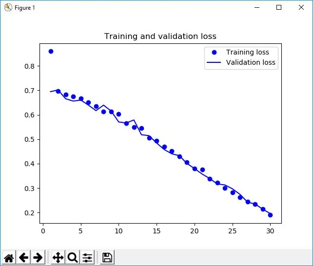
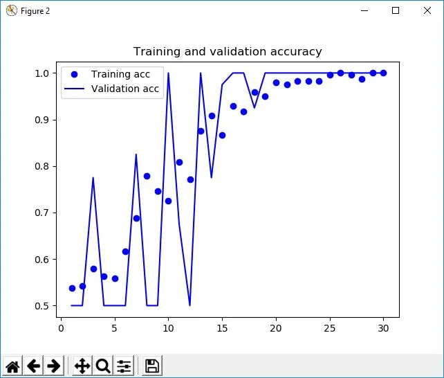
Pretty good results on the validation set, I’m sure you’ll agree!

Plotting the Accuracy and Loss

Finally, I used the following code to plot the results.

# Show plots of training loss and accuracy
loss = history.history["loss"]
val_loss = history.history["val_loss"]

acc = history.history["acc"]
val_acc = history.history["val_acc"]

epochs = range(1, len(acc) + 1)

plt.plot(epochs, loss, 'bo', label="Training loss")
plt.plot(epochs, val_loss, 'b', label="Validation loss")
plt.title("Training and validation loss")
plt.legend()

plt.figure()

plt.plot(epochs, acc, 'bo', label="Training acc")
plt.plot(epochs, val_acc, 'b', label="Validation acc")
plt.title("Training and validation accuracy")
plt.legend()

plt.show()

And here are the results.